I recently read Ewan Birney's blog post, which I found echoed a lot of my own thoughts about the use of statistical in computational biology. I thought I would compile my own similar list but for bioinformatics / computational biology in general. I have not been and in the field as long as Ewan and I certainly still have a lot to learn, particularly about statistics due to my biological background, but I have learnt some things over the last ten years, that like Ewan, I wish someone had told me long ago. The points are in no particular order.
Showing posts with label R. Show all posts
Showing posts with label R. Show all posts
Thursday, 7 July 2011

Friday, 10 December 2010
R: Basic R Skills - Splitting and Plotting
I am giving a short R course next year, so I am going to make a series of blog posts to help get my thoughts and example code in order. The aim is to introduce people with little or no experience of R to the language with self contained examples. The order of the posts are not going to reflect any order in the course, just what I feel like doing at the time.
This first post is going to deal with splitting and plotting data. It is a common occurrence to have data in such a form that you want to split the data in one column based on the data in another column. Maybe you want to split an experimental result by age or gender for example. Perhaps you want to see if there is a difference in the distribution of results in males and females. The example code below goes through one such hypothetical example.
 The figure shows the output you should get from running the code. Essentially the example is designed to illustrate the split function and the ~ (tilde) character.
The split function will do what it says, split a vector of data (A), based on another vector (B). It returns a list, with each element of the list being all of the element in A that match each element in B. For example
This first post is going to deal with splitting and plotting data. It is a common occurrence to have data in such a form that you want to split the data in one column based on the data in another column. Maybe you want to split an experimental result by age or gender for example. Perhaps you want to see if there is a difference in the distribution of results in males and females. The example code below goes through one such hypothetical example.

The split function will do what it says, split a vector of data (A), based on another vector (B). It returns a list, with each element of the list being all of the element in A that match each element in B. For example
A <- c(1,2,3,4)
B <- c("X","Y","X","Y")
sp <- split(A,B)
sp
$X
[1] 1 3
$Y
[1] 2 4
Now we have a list, and we can operate on each element of the list using the apply functions, such as lapply.
lapply(sp,sum)
$X
[1] 4
$Y
[1] 6
There are lots off different apply functions, a good introduction is here.
The other main way of splitting is using the ~ (tilde) operation. In my head I always read this as 'given', such as plot(A ~ B) is "plot A given B". This is an example of the formula notation in R, but here we are using it very simply. It essentially does the same thing as split.
Note: You actually need to do plot(A ~ factor(B)) if B isn't already a factor.
Lots of functions support the function call, such as t.test in the example, for others you can use the lapply and split version, such as for density in the example.
I also mention the aggregate function, which essentially is the same as lapply and split but seems slower on large datasets.
Wednesday, 8 December 2010
R: Using RColorBrewer to colour your figures in R
RColorBrewer is an R packages that uses the work from http://colorbrewer2.org/ to help you choose sensible colour schemes for figures in R. For example if you are making a boxplot with eight boxes, what colours would you use, or if you are drawing six lines on an x-y plot what colours would you use so you can easily distinguish the colours and look them up on a key? RColorBrewer help you to do this.
Below is some example R code that generates a few plots, coloured by RColorBrewer.
The colours are split into three group, sequential, diverging, and qualitative.
This will generate 100 colours based on the 9 from the 'Blues' palette. See image below for a contrast.
Below is some example R code that generates a few plots, coloured by RColorBrewer.
The colours are split into three group, sequential, diverging, and qualitative.
- Sequential - Light colours for low data, dark for high data
- Diverging - Light colours for mid-range data, low and high contrasting dark colours
- Qualitative - Colours designed to give maximum visual difference between classes
The main function is brewer.pal, which you simply give the number of colours you want, and the name of the palette, which you can choose from running display.brewer.all()
There are limits on the number of colours you can get, but if you want to extend the Sequential or Diverging groups you can do so with the colorRampPalatte command, for example :
There are limits on the number of colours you can get, but if you want to extend the Sequential or Diverging groups you can do so with the colorRampPalatte command, for example :
colorRampPalette(brewer.pal(9,"Blues"))(100)
This will generate 100 colours based on the 9 from the 'Blues' palette. See image below for a contrast.
 |
| From compBiomeBlog |
Friday, 18 June 2010
R: Command Line Calculator using Rscript
I currently use an awesome little bash trick to get a command line calculator that was posted on lifehacker, and that I blogged about previously.
This is really useful, however I recently stumbled upon Rscript. This comes with the standard R install and allows you to make a scripts similar to perl or bash with the shebang #!/usr/bin/Rscript, or wherever your Rscript is (you can check with a whereis Rscript command). The nice thing is that it also has a -e option for evaluating an expression at the command line, just like the perl -e for perl one liners. For example:
Rscript -e "round(runif(10,1,100),0)"
[1] 17 23 21 36 10 47 90 81 83 5
This gives you 10 random numbers uniformly distributed between 1 and 100. You can use any R functions this way, even plot for making figures.
Anyway, it seemed that Rscript would be really useful as a command line calculator too. So after a bit of playing and Googling I adapted a nice alias found in a comment on this blog post. Here it is :
So now you can type things like Calc "-log10(0.05)", whereas my above mentioned calc would just stare at me blinking, looking a bit embarrassed. You can really go to town if you like:
calc(){ awk "BEGIN{ print $* }" ;}You just add this to your .bashrc file and then you can use it just like calc 2+2.
This is really useful, however I recently stumbled upon Rscript. This comes with the standard R install and allows you to make a scripts similar to perl or bash with the shebang #!/usr/bin/Rscript, or wherever your Rscript is (you can check with a whereis Rscript command). The nice thing is that it also has a -e option for evaluating an expression at the command line, just like the perl -e for perl one liners. For example:
Rscript -e "round(runif(10,1,100),0)"
[1] 17 23 21 36 10 47 90 81 83 5
This gives you 10 random numbers uniformly distributed between 1 and 100. You can use any R functions this way, even plot for making figures.
Anyway, it seemed that Rscript would be really useful as a command line calculator too. So after a bit of playing and Googling I adapted a nice alias found in a comment on this blog post. Here it is :
alias Calc='Rscript -e "cat( file=stdout(), eval( parse( text=paste( commandArgs(TRUE), collapse=\"\"))),\"\n\")"'
So now you can type things like Calc "-log10(0.05)", whereas my above mentioned calc would just stare at me blinking, looking a bit embarrassed. You can really go to town if you like:
Calc "round(log2(sqrt(100)/exp(0.05)*(1/factorial(10))),2)"
Calc "plot(hist(rnorm(1E6),br=100))"I think I will probably keep the calc version too as it is a bit quicker, with it's lower overhead, but Calc should be useful for more complex things too.
Monday, 19 April 2010
R tip: Maximum screen width
R can be annoying in that even if you stretch your terminal or R GUI session to a whole screen width it will still only show 80 characters width. This can make wide tables really hard to read.
Use the options command width to set this parameter to what ever you like. Easy.
options(width=150)
Use the options command width to set this parameter to what ever you like. Easy.
Wednesday, 14 April 2010
R: parallel processing using multicore package
I have been meaning to look at adding some parallel processing to R as I have some scripts that are painfully slow and embarrassingly parallel. There seem to be a lot of packages around for doing parallel computing, listed here.
I decided to look at multicore as it seemed easy to implement. The core of the package is the mclapply function, which is the multi core version of lapply. Basically you install the package,
load the library,
then replace any instances of lapply in your code with mclapply it will speed up your code! Easy.
Obviously there are more complications than this and there are various options you can use, such as the number of cores to use etc.
To give a quick test:
So the elapsed time went down from 2.795 to 0.914, which is about three times faster. Not bad.
The package also contains parallel and collect functions which allow you to run any processes in parallel, then collect will recover the results when they are all finished.
I have only just started using it, but first impressions are good.
I decided to look at multicore as it seemed easy to implement. The core of the package is the mclapply function, which is the multi core version of lapply. Basically you install the package,
install.packages("multicore")
load the library,
library(multicore)
then replace any instances of lapply in your code with mclapply it will speed up your code! Easy.
Obviously there are more complications than this and there are various options you can use, such as the number of cores to use etc.
To give a quick test:
test <- lapply(1:10,function(x) rnorm(10000))
system.time(x <- lapply(test,function(x) loess.smooth(x,x)))
# user system elapsed
# 0.954 0.246 2.795
system.time(x <- mclapply(test,function(x) loess.smooth(x,x)))
# user system elapsed
# 0.896 0.898 0.914
So the elapsed time went down from 2.795 to 0.914, which is about three times faster. Not bad.
The package also contains parallel and collect functions which allow you to run any processes in parallel, then collect will recover the results when they are all finished.
I have only just started using it, but first impressions are good.
Thursday, 8 April 2010
R: heatmaps with gplots
I use heatmaps quite a lot for visualizing data, microarrays of course but also DNA motif enrichment, base composition and other things. I particular like the heatmap.2 function of the gplots package. It has a couple of defaults that are a little ugly but they are easy to remove. Here is a quick example:
First lets make some example microarray data.
Next I will just plot the most variable row/genes/whatever, this step is obviously optional but it reduces the size of the plot to make them easier to see, and normally I only care about the things that are different.
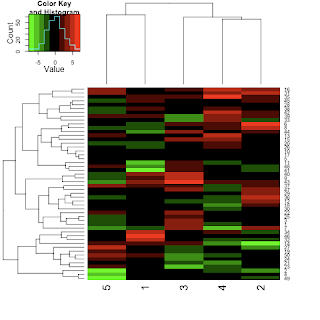
Next we load the gplots package (install it first if you do not already have it). We then simple pass the mostVariable matrix to the heatmap.2 function. The trace="none" option removes a default, which is to add a line to each column, which I find distracting. The col=greenred(10) option uses another gplots function (greenred), which simply generates a color scheme from green to red via black. You could use any color scheme here such as col=rainbow(10) or a scheme from RColorBrewer.
That is about it really for basic heatmaps.
For more advanced heatmaps, you can do other things such as adding color strips to the rows or columns to show groupings, for example:
Another useful trick is not to use the default clustering methods of heatmap.2, but use your own. For example :
 There are lots of other options too, but that is enough for today.
First lets make some example microarray data.
exampleData <- matrix(log2(rexp(1000)/rexp(1000)),nrow=200)This just makes two exponential distributions and takes the log2 ratio to make it look a bit like microarray fold changes, but this really could be able matrix of numbers.
Next I will just plot the most variable row/genes/whatever, this step is obviously optional but it reduces the size of the plot to make them easier to see, and normally I only care about the things that are different.
This just calculates the variance of each row in the matrix, then makes a new matrix of those rows that have a variance that is above the 75th percentile, so the top 25% most variable row.evar <- apply(exampleData,1,var)mostVariable <- exampleData[evar>quantile(evar,0.75),]
#install.packages("gplots")library(gplots)heatmap.2(mostVariable,trace="none",col=greenred(10))

Next we load the gplots package (install it first if you do not already have it). We then simple pass the mostVariable matrix to the heatmap.2 function. The trace="none" option removes a default, which is to add a line to each column, which I find distracting. The col=greenred(10) option uses another gplots function (greenred), which simply generates a color scheme from green to red via black. You could use any color scheme here such as col=rainbow(10) or a scheme from RColorBrewer.
That is about it really for basic heatmaps.
For more advanced heatmaps, you can do other things such as adding color strips to the rows or columns to show groupings, for example:
heatmap.2(mostVariable,trace="none",col=greenred(10),ColSideColors=bluered(5))
Another useful trick is not to use the default clustering methods of heatmap.2, but use your own. For example :
Here were are generating the ordering of the rows ourselves, in this case by the sum of the absolute values of each row. Then we turn off the clustering of the rows and the row dendrogram and get something like this:ord <- order(rowSums(abs(mostVariable)),decreasing=T)heatmap.2(mostVariable[ord,],Rowv=F,dendrogram="column",trace="none",col=greenred(10))

Friday, 26 February 2010
R tip: Finding the location of minimum and maximums
I can never remember this R command, so I am going to post it here which probably means I will always remember it and never have to look it up here again.
I sometimes want to find the location of a minimum or maximum value in a vector, so I can look up the corresponding position in another vector, or column or something. You can just use order but that is a bit clunky and more prone to error, so what you really need is which.min and which.max.
x <- sample(1:100,20)
which.min(x)
x <- matrix(sample(1:100,20),nrow=10)
x[which.min(x[,2]),1]
Not exactly earth-shatteringly useful but better than:
x <- matrix(sample(1:100,20),nrow=10)
x[order(x[,2])[1],1]
Or is it? Now I write that, it is actually less characters than which.min. Oh well.
I sometimes want to find the location of a minimum or maximum value in a vector, so I can look up the corresponding position in another vector, or column or something. You can just use order but that is a bit clunky and more prone to error, so what you really need is which.min and which.max.
x <- sample(1:100,20)
which.min(x)
x <- matrix(sample(1:100,20),nrow=10)
x[which.min(x[,2]),1]
Not exactly earth-shatteringly useful but better than:
x <- matrix(sample(1:100,20),nrow=10)
x[order(x[,2])[1],1]
Or is it? Now I write that, it is actually less characters than which.min. Oh well.
Monday, 21 December 2009
Sweave in TeXShop
I love using TeXShop for GUI editing of LaTeX and particularly Sweave documents, but it is a pain not being able to get it to automatically generate the pdf output. Luckily I found this post which explains how to add a Sweave engine.
Basically, make a file called Sweave.engine in
The just select Sweave as the document type and Typeset now works, easy.
Basically, make a file called Sweave.engine in
~/Library/TeXShop/Engines/
#!/bin/bash

export PATH=$PATH:/usr/texbin:/usr/local/bin
R CMD Sweave "$1"
pdflatex -interaction batchmode "${1%.*}"
pdflatex -interaction batchmode "${1%.*}"
The just select Sweave as the document type and Typeset now works, easy.
Tuesday, 17 November 2009
R tip: Extracting median from survfit object
A colleague wanted to extract the median value from a survival analysis object, which turned out to be a pain as the value is not stored in the object, but calculated on the fly by a print method.
> library(survival)But how do you get the median value? Some googling came up with this link. The answer is rather clunky:
> fit <- coxph(Surv(time, status) ~ x, data=aml)
> survfit(fit)
Call: survfit(formula = fit)
records n.max n.start events median 0.95LCL 0.95UCL
23 23 23 18 30 18 45
> x <- read.table(textConnection(capture.output(survfit(fit))),skip=2,header=TRUE)
> x$median
[1] 30
Friday, 23 October 2009
RSPerl : Using R from within Perl
Some things I write in perl some in R, sometime I use perl to write R and run R. One thing that I find very useful is the functionality of RSPerl which enables you to call R functions from within perl and on perl variables. It can also call perl from R, though I have no idea why you would want to do this.
My main use is to carry out statistical tests on the results of things carried out in. For example I use perl to run patser to count the number of hits to a position weight matrix in a test sequence and a background sequences, then I use RSPerl to calculate the p-value via the binomial test (binom.test function).
It was a pain to setup, as I had to recompile R and install various modules in the correct places and setup some environment variables. Once working though it is a great tool. You can even use R's great graphical capabilities to automatically generate figures from data in perl variables.
perl -e 'use R;&R::initR("--silent","--vanilla");&R::eval("r <- rnorm(100);plot(r,pch=20)");'
This one plots a histogram of the length of perl scripts!
for f in *.pl; do wc -l ${f}|cut -f 1 -d " "; done | perl -ne 's/\n/,/g;print;' |perl -ne 'use R;&R::initR("--silent","--vanilla");chop;&R::eval("hist(c($_),main=\"File Lengths\",xlab=\"Number of Lines\")");sleep 10'
RSPerl
My main use is to carry out statistical tests on the results of things carried out in. For example I use perl to run patser to count the number of hits to a position weight matrix in a test sequence and a background sequences, then I use RSPerl to calculate the p-value via the binomial test (binom.test function).
It was a pain to setup, as I had to recompile R and install various modules in the correct places and setup some environment variables. Once working though it is a great tool. You can even use R's great graphical capabilities to automatically generate figures from data in perl variables.
perl -e 'use R;&R::initR("--silent","--vanilla");&R::eval("r <- rnorm(100);plot(r,pch=20)");'
This one plots a histogram of the length of perl scripts!
for f in *.pl; do wc -l ${f}|cut -f 1 -d " "; done | perl -ne 's/\n/,/g;print;' |perl -ne 'use R;&R::initR("--silent","--vanilla");chop;&R::eval("hist(c($_),main=\"File Lengths\",xlab=\"Number of Lines\")");sleep 10'
RSPerl
Tuesday, 18 August 2009
R Coding Style Guide
I was sent this R style guide, and think it looks like it might be a good idea. R can be pretty difficult to read, especially someone else's.
Monday, 27 July 2009
biomaRt
I use R and Bioconductor for most of my work. I am also increasingly replacing things I would have done before in Perl with R. One such example of this is the Bioconductor module biomaRt.
As the name suggest it allows for access to BioMart via R. BioMart is a method of accessing large online databases such as Ensembl. For example you may want to convert gene IDs from Entrez to Symbols, or retrieve 5kb upstream from the transcription start site of a list of genes etc etc. There are lots of things you can do with it.
biomaRt lets you do all this via R. This is particular appealing to me as I do differential gene expression analysis in R, so I have lists of genes already in R objects which I can retrieve lots of information about. Maybe I want all the GO annotations for a gene list, or to find a list of any SNPs within the coding region or something.
Anyway it is pretty useful, the documentation isn't bad either.
http://www.bioconductor.org/packages/release/bioc/html/biomaRt.html
To give a brief example of how it works:
The functions
You can also access lots of other databases, not just Ensemble as shown here.
Enjoy.
As the name suggest it allows for access to BioMart via R. BioMart is a method of accessing large online databases such as Ensembl. For example you may want to convert gene IDs from Entrez to Symbols, or retrieve 5kb upstream from the transcription start site of a list of genes etc etc. There are lots of things you can do with it.
biomaRt lets you do all this via R. This is particular appealing to me as I do differential gene expression analysis in R, so I have lists of genes already in R objects which I can retrieve lots of information about. Maybe I want all the GO annotations for a gene list, or to find a list of any SNPs within the coding region or something.
Anyway it is pretty useful, the documentation isn't bad either.
http://www.bioconductor.org/packages/release/bioc/html/biomaRt.html
To give a brief example of how it works:
library(biomaRt)This code will retrieve 5kb upstream of the transcription start sites of the two genes listed in the 'ids' list (though this could be a much longer list). It will then generate an html output file with information about these genes. Simple and effective.
ids <- c("7157","3845") ensembl = useMart("ensembl", dataset = "hsapiens_gene_ensembl") seqs <- getSequence(id = ids, type = "entrezgene", seqType = "transcript_flank", upstream = 5000, mart = ensembl) seqs <- getSequence(id = ids, type = "entrezgene", seqType = "transcript_flank", upstream = 5000, mart = ensembl) exportFASTA(sequences=seqs,file="example.fas") library(xtable) results <- getGene(id=ids,type="entrezgene",mart=ensembl) print(xtable(results),type="html",file="Example.html")
The functions
- listAttributes(ensembl)
- listFilters(ensembl)
You can also access lots of other databases, not just Ensemble as shown here.
Enjoy.
Subscribe to:
Posts (Atom)